|
||||||||||||||||||||||||||||||||||||||||||||||||||||||||
|
||||||||||||||||||||||||||||||||||||||||||||||||||||||||
Title: Why Use DSP?
Author: David Skolnick and Noam Levine
Company: Analog Devices
Having heard a lot about digital signal processing (DSP) technology, you may have wanted to find out what can be done with DSP, investigate why DSP is preferred to analog circuitry for many types of operations, and discover how to learn enough to design your own DSP system. This article, the first of a series, is an opportunity to take a substantial first step towards finding answers to your questions. This series is an introduction to DSP topics from the point of view of analog system designers seeking additional tools for handling analog signals. Designers reading this series can learn about the possibilities of DSP to deal with analog signals and where to find additional sources of information and assistance.
What is [a] DSP? In brief, DSPs are processors or microcomputers whose hardware, software, and instruction sets are optimized for high-speed numeric processing applications an essential for processing digital data representing analog signals in real time. What a DSP does is straightforward. When acting as a digital filter, for example, the DSP receives digital values based on samples of a signal, calculates the results of a filter function operating on these values, and provides digital values that represent the filter output; it can also provide system control signals based on properties of these values. The DSPs high-speed arithmetic and logical hardware is programmed to rapidly execute algorithms modelling the filter transformation.
The combination of design elements arithmetic operators, memory
handling, instruction set, parallelism, data addressing that provide
this ability forms the key difference between DSPs and other kinds of processors.
Understanding the relationship between real-time signals and DSP calculation
speed provides some background on just how special this combination is.
The real-time signal comes to the DSP as a train of individual samples
from an analog-to-digital converter (ADC). To do filtering in real-time,
the DSP must complete all the calculations and operations required for
processing each sample (usually updating a process involving many previous
samples) before the next sample arrives. To perform high-order filtering
of real-world signals having significant frequency content calls for really
fast processors.
WHY USE A DSP?
To get an idea of the type of calculations a DSP does and get an idea
of how an analog circuit compares with a DSP system, one could compare
the two systems in terms of a filter function. The familiar analog filter
uses resistors, capacitors, inductors, amplifiers. It can be cheap and
easy to assemble, but difficult to calibrate, modify, and maintain
a difficulty that increases exponentially with filter order. For many purposes,
one can more easily design, modify, and depend on filters using a DSP because
the filter function on the DSP is software-based, flexible, and repeatable.
Further, to create flexibly adjustable filters with higher-order response
requires only software modifications, with no additional hardware
unlike purely analog circuits. An ideal bandpass filter, with the frequency
response shown in Figure 1, would have the following characteristics:
As Figure 1 shows, an analog approach using second-order filters
would require quite a few staggered high-Q sections; the difficulty of
tuning and adjusting it can be imagined.
`
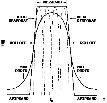
Figure 1. An ideal bandpass filter and second-order approximations.
With DSP software, there are two basic approaches to filter design: finiteimpulse response (FIR) and infinite impulse response (IIR). The FIR filters time response to an impulse is the straightforward weighted sum of the present and a finite number of previous input samples. Having no feedback, its response to a given sample ends when the sample reaches the end of the line (Figure 2). An FIR filters frequency response has no poles, only zeros. The IIR filter, by comparison, is called infinite because it is a recursive function: its output is a weighted sum of inputs and outputs. Since it is recursive, its response can continue indefinitely. An IIR filter frequency response has both poles and zeros.
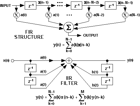
Figure 2. Filter equations and delay-line representation.
Approximating an ideal filter consists of applying a transfer function with appropriate coefficients and a high enough order, or number of taps (considering the train of input samples as a tapped delay line). Figure 3 shows the response of a 90-tap FIR filter compared with sharp-cutoff Chebyshev filters of various orders. The 90-tap example suggests how close the filter can come to approximating an ideal filter. Within a DSP system, programming a 90-tap FIR filter like the one in Figure 3 is not a difficult task. By comparison, it would not be cost-effective to attempt this level of approximation with a purely analog circuit. Another crucial point in favor of using a DSP to approximate the ideal filter is long-term stability. With an FIR (or an IIR having sufficient resolution to avoid truncation-error buildup), the programmable DSP achieves the same response, time after time. Purely analog filter responses of high order are less stable with time.
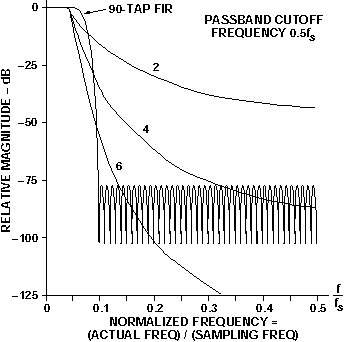
Figure 3. 90-tap FIR filter response compared with those of sharp cutoff Chebyshev filters.
Mathematical transform theory and practice are the core requirement
for creating DSP applications and understanding their limits. This article
series walks through a few signal-analysis and -processing examples to
introduce DSP concepts. The series also provides references to texts for
further study and identifies software tools that ease the development of
signal-processing software.
SAMPLING REAL-WORLD
SIGNALS
Real-world phenomena are analog the continuously changing energy
levels of physical processes like sound, light, heat, electricity, magnetism.
A transducer converts these levels into manageable electrical voltage and
current signals, and an ADC samples and converts these signals to
digital for processing. The conversion rate, or sampling frequency, of
the ADC is critically important in digital processing of real-world signals.
This sampling rate is determined by the amount of signal information that is needed for processing the signals adequately for a given application. In order for an ADC to provide enough samples to accurately describe the real-world signal, the sampling rate must be at least twice the highest-frequency component of the analog signal. For example, to accurately describe an audio signal containing frequencies up to 20 kHz, the ADC must sample the signal at a minimum of 40 kHz. Since arriving signals can easily contain component frequencies above 20 kHz (including noise), they must be removed before sampling by feeding the signal through a low-pass filter ahead of the ADC. This filter, known as an anti-aliasing filter, is intended to remove the frequencies above 20 kHz that could corrupt the converted signal.
However, the anti-aliasing filter has a finite frequency rolloff, so additional bandwidth must be provided for the filters transition band. For example, with an input signal bandwidth of 20 kHz, one might allow 2 to 4 kHz of extra bandwidth.
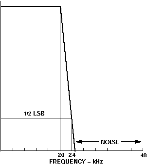
Figure 4. Antialiasing filter ideal response.
Processing speed at a required sample rate is influenced by algorithm complexity. As a rule, the DSP needs to finish all operations relating to the first sample before receiving the second sample. The time between samples is the time budget for the DSP to perform all processing tasks. For the audio example, a 48-kHz sampling rate corresponds to a 20.833-µs sampling interval. Figure 5 relates the analog signal and digital sampling rate.
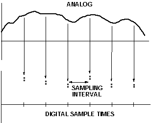
Figure 5. Sampling train and processing time.
Next consider the relation between the speed of the DSP and complexity of the algorithm (the software containing the transform or other set of numeric operations). Complex algorithms require more processing tasks. Because the time between samples is fixed, the higher complexity calls for faster processing. For example, suppose that the algorithm requires 50 processing operations to be performed between samples. Using the previous examples 48-kHz sampling rate (20.833-µs sampling interval), one can calculate the minimum required DSP processor speed, in millions of operations per second (MOPS) as follows:

Thus if all of the time between samples is available for operations
to implement the algorithm, a processor with a performance level of 2.4
MOPS is required. Note that the two common ratings for DSPs, based on operations
per second (MOPS) and instructions per second (MIPS), are not the same.
A processor with a 10-MIPS rating that can perform 8 operations per instruction
has basically the same performance as a faster processor with a 40 MIPS
rating that can only perform 2 operations per instruction.
SAMPLING VARIOUS REAL-WORLD SIGNALS
There are two basic ways to acquire data, either one sample at a time
or one frame at a time (continuous processing vs. batch processing). Sample-based
systems, like a digital filter, acquire data one sample at a time. As shown
in Figure 6, at each tick of the clock, a sample comes into the system
and a processed sample is output. The output waveform develops continuously.
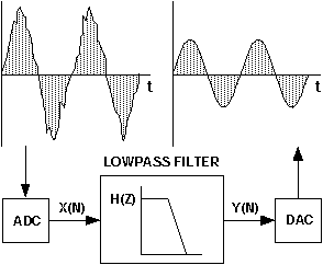
Figure 6. Example of continuous processing of samples in digital filter.
Frame-based systems, like a spectrum analyzer, which determines the frequency components of a time-varying waveform, acquire a frame (or block of samples). Processing occurs on the entire frame of data and results in a frame of transformed data, as shown in Figure 7.
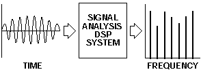
Figure 7. Example of batch processing of a block of data.
For an audio sampling rate of 48 kHz, a processor working on a frame
of 1024 samples has a frame acquisition interval of 21.33 ms (i.e., 1024
x 20.833 µs = 21.33 ms). Here the DSP has 21.33 ms to complete all
the required processing tasks for that frame of data. If the system handles
signals in real time, it must not lose any data; so while the DSP is processing
the first frame, it must also be acquiring the second frame. Acquiring
the data is one area where special architectural features of DSPs come
into play: Seamless data acquisition is facilitated by a processors flexible
data-addressing capabilities in conjunction with its direct memory-accessing
(DMA) channels.
RESPONDING TO REAL-WORLD SIGNALS
One cannot assume that all the time between samples is available for
the execution of processing instructions. In reality, time must be budgeted
for the processor to respond to external devices, controlling the flow
of data in and out. Typically, an external device (such as an ADC) signals
the processor using an interrupt. The DSPs response time to that interrupt,
or interrupt latency, directly influences how much time remains
for actual signal processing.
Interrupt latency (response delay) depends on several factors; the most dominant is the DSP architectures instruction pipelining. An instruction pipeline consists of the number of instruction cycles that occur between the time an interrupt is received and the time that program execution resumes. More pipeline levels in a DSP result in longer interrupt latency. For example, if a processor has a 20-ns cycle time and requires 10 cycles to respond to an interrupt, 200 ns elapse before it executes any signal-processing instructions.
When data is acquired one sample at a time, this 200-ns overhead will
not hurt if the DSP finishes the processing of each sample before the next
arrives. When data is acquired sample-by-sample while processing a frame
at a time, however, an interrupted system wastes processor instruction
cycles. For example, a system with a 200-ns interrupt response time running
a frame-based algorithm, such as the FFT, with a frame size of 1024 samples,
would require 204.8 µs of overhead. That amounts to more than 10,000
instruction cycles wasted to latency productive time when the DSP
could be performing signal processing. This waste is easy to avoid in DSPs
having architectural features such as DMA and dual memory access; they
let the DSP receive and store data without interrupting the processor.
DEVELOPING A DSP SYSTEM
Having discussed the role of the processor, the ADC, the anti-aliasing
filter, and the timing relationships between these components, it is time
to look at a complete DSP system. Figure 8 shows the building blocks of
a typical DSP system that could be used for data acquisition and control.
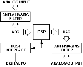
Figure 8. Putting together elements of a DSP system.
Note how few components make up the DSP system, because so much of the systems functionality comes from the programmable DSP. Converters funnel data into and out of the DSP; the ADC timing is controlled by a precise sampling clock. To simplify system design, many converter devices available today combine some or all of the following: an A/D converter, a D/A converter, a sampling clock, and filters for anti-aliasing and anti-imaging. The clock oscillator in these types of I/O components is separately controlled by an external crystal. Here are some important points about the data flow in this sort of DSP system:
Analog Input: The analog signal is appropriately band-limited by the anti-aliasing filter and applied to the input of the ADC. At the selected sampling time, the converter interrupts the DSP processor and makes the digital sample available. The choice between serial and parallel interfacing between the ADC and DSP depends on the amount of data, design complexity trade-offs, space, power, and price.
Digital Signal Processing: The incoming data is handled by the DSPs algorithm software. When the processor completes the required calculations, it sends the result to the DAC. Because the signal processing is programmable, considerable flexibility is available in handling the data and improving system performance with incremental programming adjustments.
Analog Output: The DAC converts the DSPs output into the desired analog output at the next sample clock. The converters output is smoothed by a low-pass, anti-imaging filter (also called a reconstruction filter), to produce the reconstructed analog signal.
Host Interface: An optional host interface lets the DSP communicate
with external systems, sending and receiving data and control information.
REVIEW AND PREVIEW
The goal of this article has been to provide an overview of major DSP
design concepts and explain some of the reasons why a DSP is better suited
that analog circuitry for some applications. The issues introduced in this
article include:
References
Higgins, R. J. Digital Signal Processing in VLSI,
Englewood Cliffs, NJ: Prentice Hall, 1990. DSP basics. Includes a wide-ranging
bibliography. Available for purchase from ADI.
Mar, A., ed. Digital Signal Processing Applications Using the ADSP-2100 Family Volume 1, Englewood Cliffs, NJ: Prentice Hall, 1992. Available for purchase from ADI.
Mar, A., Babst, J., eds. Digital Signal Processing Applications Using the ADSP-2100 Family Volume 2, Englewood Cliffs, NJ: Prentice Hall, 1994. Available for purchase from ADI.
Dearborn, G., ed. Digital Signal Processing Applications Using the ADSP-21000 Family Volume 1, Norwood, MA: Analog Devices, Inc., 1994. Available for purchase from ADI.
*Mar, A., Rempel, H., eds. ADSP-2100 Family Users Manual, Norwood, MA: Analog Devices, Inc., 1995. Free.
Mar, A., Rempel, H., eds. ADSP-21020 Family Users Manual, Norwood, MA: Analog Devices, Inc., 1995. Free.
*Rempel, H., ed. ADSP-21060/62 SHARC Users Manual,
Norwood, MA: Analog Devices, Inc., 1995. Free.